When you activate a table you can configure its settings, which are inherited by metrics that are based on the table. You can override these settings on a per-metric basis as needed.

Note that these settings are not inherited by SQL metrics. With a SQL metric, you manage its settings via a combination of configuration options and SQL.

Except for Query Scope, table settings can be changed after you save the table configuration. Any changes will be inherited by any metrics that are inheriting settings.

Data Collection settings

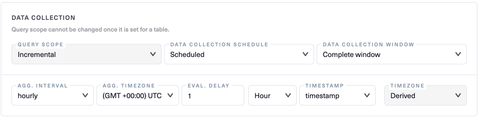
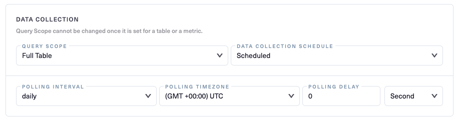
The Data Collection settings you can select depend on how you set Query Scope, which can only be set for a table when you first configure it— you can't change this setting after you save the table's configuration. However, if you override inherited table settings in a metric, you can change the Query Scope for the metric.

If Query Scope is set to Incremental, your form will have the fields shown below:

If Query Scope is set to Full Table, your form will instead have the fields shown below.

The various Data Collection settings are described on the following pages:

• Query scope
• Data collection schedule
• Data collection window
• Aggregation interval
• Polling interval
• Aggregation time zone
• Polling timezone
• Evaluation delay
• Polling delay
• Timestamp
• Timestamp timezone
• Partitions