
SQL metrics
Lightup's No-code and Low-code Data Quality metrics cover a significant amount of data quality requirements. However, there are times when a SQL metric is still need to be used:
- Multi-column Aggregation
- CASE statements
- Multiple JOINs
- Sub-queries or CTEs
- Complex WHERE logic (i.e. OR or () are required)
Before starting with a SQL-based metric, it is important to understand what the desired outcome of the metric is and format the SQL query to get the outcome which Lightup is expecting.
Know Before You SQL
Format SQL for Lightup's Expected Outcome
The essential outcome of a SQL metric in Lightup is a single, numerical data point for a given interval window (5 Minutes, Hourly, Daily, and so on).
Example: Daily sum of values in a column should result in a single numerical data point per day
Therefore, the fundamental SQL requirements are a SELECT statement, an Aggregation function in the SELECT statement, and a GROUP BY.
The following SQL is an example of getting the count orders per hour:
SELECT
	DATE_TRUNC('HOUR', order_timestamp) as "hourly_orders",
  COUNT(*)
FROM
  customer_orders_table
WHERE
	order_timestamp >= {start_ts}
  AND order_timestamp < {end_ts}
GROUP BY
  hourly_orders
Notice how the timestamp had to be truncated to the hour to get a total count of orders to match the aggregation interval of an hour. The outcome of this query should get a maximum of 1 data point per hour.
The following SQL adds a slicing column to the previous SQL query:
SELECT
	DATE_TRUNC('HOUR', order_timestamp) as "hourly_orders",
  city,
  COUNT(*)
FROM
  customer_orders_table
WHERE
	order_timestamp >= {start_ts}
  AND order_timestamp < {end_ts}
GROUP BY
  hourly_orders,
  city
By adding the City column in the SELECT and GROUP BY statements, Lightup will be able to slice the hourly count by distinct city value. In this scenario, if there are 10 cities, then Lightup expects a maximum of 1 data point per hour, per city.
Lightup Variables for Incremental Metrics
Also, in both of these SQL queries, there is a WHERE clause that includes a very specific setup of parameters and operators:
-
For an Incremental Metric, Lightup will need to provide the start and end time for the desired aggregation interval. In the case of an Hourly interval, Lightup will give the beginning of the hour for
{start_ts}and the beginning of the next hour for{end_ts} -
The operator for
{start_ts}needs to be>=to get all records associated to the beginning of the hour. Whereas the operator for{end_ts}needs to be<in order to get all records associated to the desired hour- If the
=operator is used for both, then the data point could be double-counting the records at the end of one hour and the beginning of the next hour - For example:
timestamp order city 01-01-2024 11:00:00 817473529374242 Tampa 01-01-2024 11:00:00 124789092831237 Sioux Falls 01-01-2024 12:00:00 423198128341982 Dallas 01-01-2024 12:00:00 798429841794712 Nashville 01-01-2024 13:00:00 3123172874812748 Tampa 01-01-2024 13:00:00 019839817248298 Salt Lake City - In the above table, if the query is used to count all records with a start time >= 11:00:00 and an end time <= 12:00:00, then the count would return 4. However, if the start and end times in the query are increased an hour to 12:00:00 and 13:00:00, then the count would be 4, which would double-count the records at 12:00:00
- If the
Available variables for the incremental SQL metric are:
| Variable | Outcome | Example |
|---|---|---|
| {start_ts}/{end_ts} | Timestamp | 2023-04-24 06:00:10 |
| {start_date}/{end_date} | Date | 2024-02-10 |
| {start_datetime}/{end_datetime} | Datetime | 2024-01-02T01:00:00 |
These variables need to match the expected outcome of the column that they are being used on (i.e. Date column cannot use {start_ts}).
Full Table SQL
If the SQL query is intended to get an aggregate outcome of all records in a table, this is where a Full Table would be used:
SELECT
  city,
  COUNT(*)
FROM
  customer_orders_table
GROUP BY
  city
This SQL shows how to get every order that each city has ever had. Depending on the polling interval for the Full Table query, Lightup will expect a maximum of one data point per polling interval window.
Timezones
In order for Lightup to execute a metric on the desired date range at the desired time, timezones must be correct. In the case of SQL metrics, there are multiple places for timezones to be specified and used:
- Aggregation Timezone is the timezone Lightup uses for the aggregation window and the scheduled execution. If the Evaluation Delay of a daily metric is 2 Hours, then Lightup will execute the metric collection at 2 am according to the Aggregation Timezone
- Timestamp Timezone is the timezone related to the timestamp that the SQL query returns.
If the Timezones are not aligned correctly, then you may get the following errors depending on the kind of mis-match:
Please review the SQL. The following rows have unexpected timestamps (epoch in seconds) and slicing values that do not match the configured aggregation timezone and slice
or Please review the SQL. The configured aggregation interval of {...} seconds does not match with the time truncation interval of {..} seconds in SQL. The following rows have unexpected timestamps (epoch in seconds) that do not match the configured aggregation timezone {...}
or Please review the SQL. Duplicate timestamp (epoch in seconds) in row {row1_in_json} and row {row2_in_json}
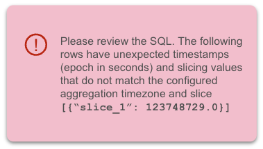
Please make sure that the timezone of the timestamp in the SQL query is correct aligned with what is in the metric configuration. One way of making sure this is correct is by leveraging a timezone conversion function in the SQL to convert the timestamp to a UTC timezone before it is returned to Lightup.
Create a SQL metric
Note that blob storage datasources (AWS S3, Azure) currently do not support SQL metrics.
-
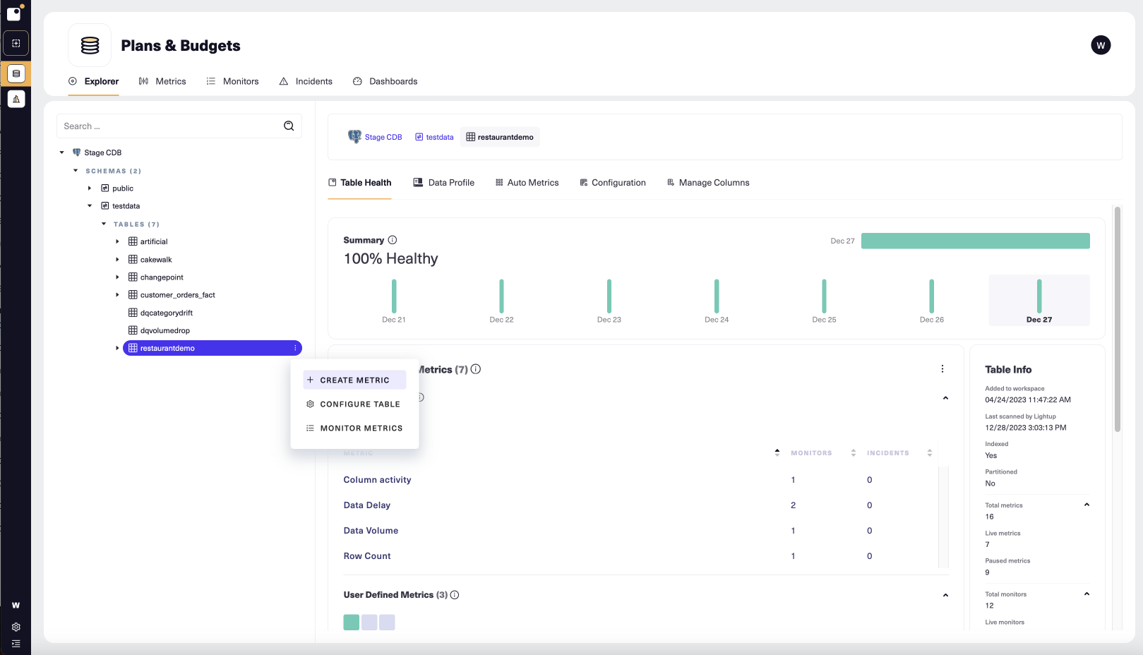
In the Explorer tree, select the data asset that you want to measure.
-
On the asset's Explorer menu select + Create Metric:
-
The metric configuration form opens. Set Metric type to SQL.
-
Enter a Metric name.
-
By default, new metrics go Live shortly after you create them. If you want the metric to start off paused, under Metric status, set Status to Paused.
-
If desired, change the value of Quality dimension. Each data quality metric measures one dimension of data quality: accuracy, completeness, timeliness, or (if none of these applies), custom. You can sort and filter your metrics by dimension, and you can view them summarized by dimension in a data quality dashboard.
-
Select Next to proceed to Step 2 (Configure Metric).
- Under Select data asset specify the data asset under which your metric will appear in the Explorer tree. This does not have an effect on the metric's source, just where it appears in the Explorer tree.
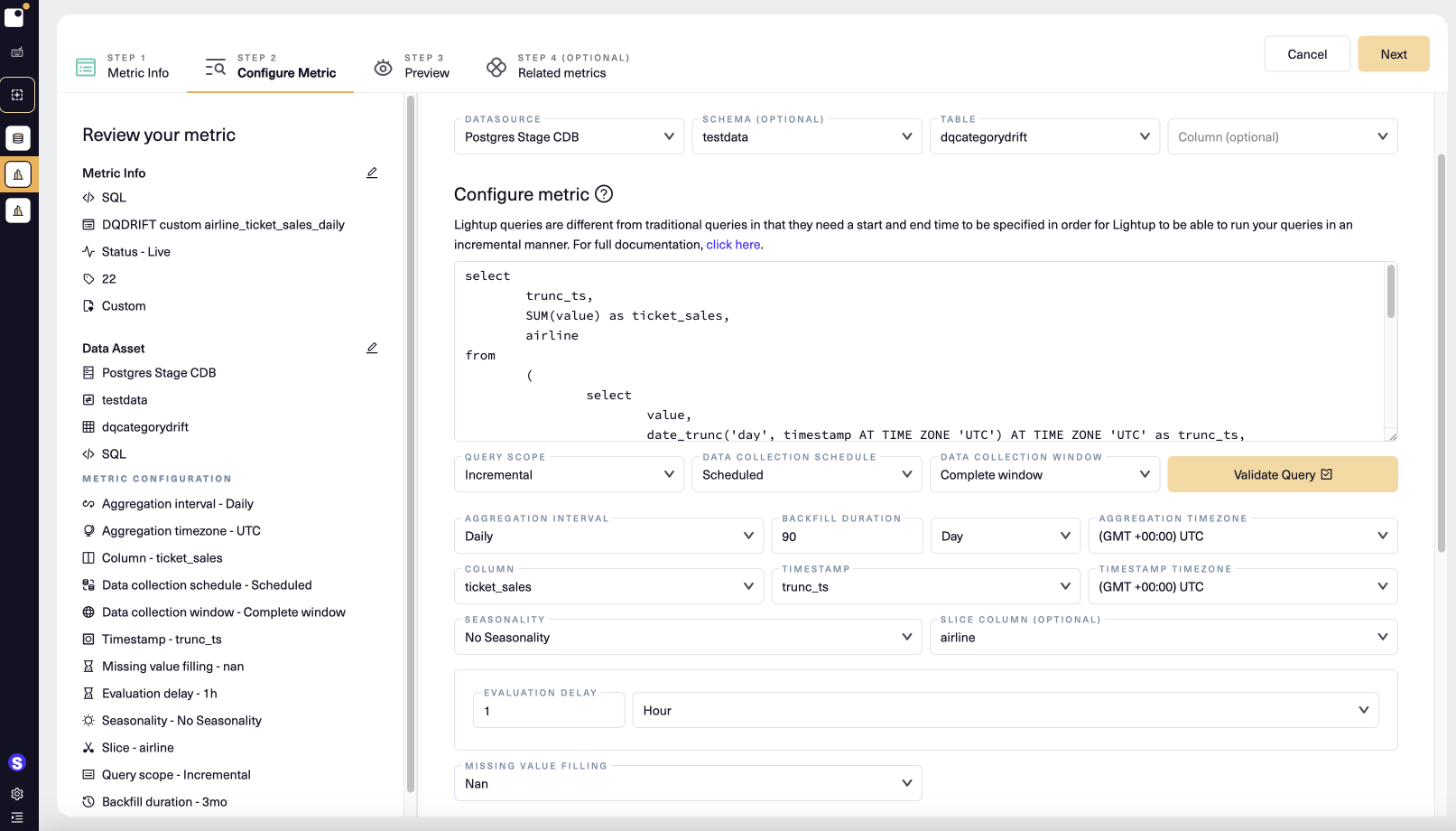
- Enter your SQL in the Custom SQL box. To produce a metric, your SQL clauses must have certain elements:
- Your SQL must SELECT at least two values, the timestamp and the aggregated metric value that you want the metric to compute. After validating the query, you will have the opportunity to select this timestamp as your timestamp, and select the metric value as the column. The timestamp will become the X-axis of your metric chart and the aggregated metric value will become the y-axis of your metric chart. If you are creating a sliced metric, you will additionally need the slice column in your SELECT.
- The WHERE clause must specify a date range using the time-based column and two tags: one producing the start of the range and another for the end of the range. These tags reflect the kind of time-based column you have: (1) use {start_ts} and {end_ts} for a timestamp column, (2) use {start_date} and {end_date} for a date column, and (3) use {start_datetime} and {end_datetime} for a datetime column.
- The timestamp in your SELECT must match the aggregation interval that you choose in the drop down selection after you click Validate Query. For example, if your metric does a SELECT of a date, you cannot set Aggregation Interval to hourly.
- Your SQL must GROUP BY the timestamp column.
- If you want to create a sliced metric, you must add a GROUP BY clause on the intended slice columns. You can then choose them as the slice column after you validate your SQL in step 3 (the next numbered item, below). Note that the slice column can't include the column with aggregated metric values in your SELECT clause.
- Note that if you want your SQL metric's Query Scope to be Full Table, the query requirements change.
- The SELECT clause doesn't need to select a timestamp.
- The WHERE clause doesn't need start and end tags.
- See below for SQL examples for each supported datasource.
- When your SQL is ready, select Validate Query. If the query validates, a number of other fields in the form become active.
- Because a SQL metric doesn't inherit Data Collection settings, you must set them. First, set Query Scope— your choice determines which other Data Collection settings appear.
| Data Collection settings | Query Scope |
|---|---|
| Data collection schedule | Incremental or Full Table |
| Data collection window | Incremental only |
| Aggregation interval | Incremental only |
| Aggregation time zone | Incremental only |
| Evaluation delay | Incremental only |
| Polling interval | Full Table only |
| Polling timezone | Full Table only |
| Polling delay | Full Table only |
| Timestamp | Incremental only |
| Timestamp timezone | Incremental only |
- Set Column to the aggregated metric value from your SELECT statement (the value the metric will track).
- If your metric has Incremental query scope, set Timestamp to the timestamp in your SELECT statement. You may need to specify the Timestamp Timezone as well, depending on the timestamp format. If your timestamp's format includes the time zone, Timestamp Timezone is not editable and reads Derived.
- If your SQL includes a GROUP BY clause on a non-timestamp column, select that column as your Slice Column.
- Optionally:
- Add seasonality
- Choose a missing value filling
- Adjust the backfill duration
- Add a failing records query
- Add tags
- If your table has a date-based partition column, you can optimize your query to query only the partitions where the data resides
SQL examples
SELECT
	date_trunc('hour', "timestamp") AS "event_ts",
	count(*) AS "cnt"
FROM
	"lightup_demo"."customer_orders_fact"
WHERE
	"timestamp" >= {start_ts}
	AND "timestamp" < {end_ts}
GROUP BY
	1
SELECT
datetime_trunc(`Test_Time`, HOUR) AS `event_ts`,
count(*) AS `cnt`
FROM
`for_test_data_cache_v2.h06bbf7787854074cca66b9c8e3397593`
WHERE
`Test_Time` >= {start_ts}
AND `Test_Time` < {end_ts}
GROUP BY
1SELECT
DATE_TRUNC('hour', `timestamp`) AS `event_ts`,
count(*) AS `cnt`
FROM
`lightup_demo`.`customer_orders_fact`
WHERE
`datehour` >= {start_partition}
AND `datehour` < {end_partition}
AND `timestamp` >= {start_ts}
AND `timestamp` < {end_ts}
GROUP BY
1SELECT
"timestamp",
AVG("order_value") AS "order_value"
FROM
(
SELECT
DATE_TRUNC('hour', "timestamp") AS "timestamp",
"order_value"
FROM
"lightup_redshift.testdb.producer"."customer_orders_fact"
WHERE
"timestamp" >= TO_TIMESTAMP(1696442400.0)
AND "timestamp" < TO_TIMESTAMP(1696957200.0)
) AS t
GROUP BY
"timestamp"
ORDER BY
"timestamp"SELECT
DATE_TRUNC('hour', `timestamp`) AS `event_ts`,
count(*) AS `cnt`
FROM
`lightup_demo`.`customer_orders_fact`
WHERE
`datehour` >= {start_partition}
AND `datehour` < {end_partition}
AND `timestamp` >= {start_ts}
AND `timestamp` < {end_ts}
GROUP BY
1SELECT
date_trunc('hour', "timestamp") AS "event_ts",
CAST(COUNT(*) AS INT) AS "cnt"
FROM
"from_teradata"."customer_orders_fact"
WHERE
"timestamp" >= {start_ts}
AND "timestamp" < {end_ts}
GROUP BY
1SELECT
"timestamp" AS "event_ts",
count(*) AS "cnt"
FROM
(
SELECT
dateadd(HOUR, datediff(HOUR, 0, "timestamp"), 0) AS "timestamp"
FROM
"testdata"."customer_orders_fact"
WHERE
"timestamp" >= {start_ts}
AND "timestamp" < {end_ts}
) AS t
GROUP BY
"timestamp"SELECT
`timestamp`,
MIN(`order_value`) AS `order_value`
FROM
(
SELECT
UNIX_TIMESTAMP(
CONVERT_TZ(
DATE_FORMAT(
CONVERT_TZ(`timestamp`, 'UTC', 'UTC'),
'%Y-%m-%d %H:00:00'
),
'UTC',
'UTC'
)
) AS `timestamp`,
`order_value`
FROM
testdata.customer_orders_fact
WHERE
`timestamp` >= '2023-10-10 16:00:00.000000'
AND `timestamp` < '2023-10-10 17:00:00.000000'
) AS t
GROUP BY
`timestamp`
ORDER BY
`timestamp`SELECT
"timestamp" AS "event_ts",
COUNT(*) AS "cnt"
FROM
(
SELECT
ROUND(
(
CAST(
SYS_EXTRACT_UTC(
FROM_TZ(
CAST(
TRUNC("timestamp" AT TIME ZONE 'UTC', 'HH24') AS TIMESTAMP
),
'UTC'
)
) AS DATE
) - DATE '1970-01-01'
) * 86400
) AS "timestamp"
FROM
"lightup_demo"."customer_orders_fact"
WHERE
"timestamp" >= {start_ts}
AND "timestamp" < {end_ts}
)
GROUP BY
"timestamp"SELECT
date_trunc('hour', "timestamp") AS "event_ts",
count(*) AS "cnt"
FROM
"testdata"."customer_orders_fact"
WHERE
"timestamp" >= {start_ts}
AND "timestamp" < {end_ts}
GROUP BY
1SELECT
date_trunc('hour', "timestamp") AS "event_ts",
count(*) AS "cnt"
FROM
"testdata"."rummy"
WHERE
"timestamp" >= {start_ts}
AND "timestamp" < {end_ts}
GROUP BY
1SELECT
date_trunc('HOUR', "LAST_UPDATED_DATE") AS "event_ts",
count(*) AS "cnt"
FROM
"PUBLIC"."CT_US_COVID_TESTS"
WHERE
"LAST_UPDATED_DATE" >= {start_ts}
AND "LAST_UPDATED_DATE" < {end_ts}
GROUP BY
1SELECT
"timestamp" AS "event_ts",
COUNT(*) AS "cnt"
FROM
(
SELECT
(
(
CAST(
(
CAST("timestamp" AS TIMESTAMP WITH TIME ZONE) AT TIME ZONE 'GMT'
) AS DATE AT TIME ZONE 'GMT'
) - DATE '1970-01-01'
) * 86400 + (
EXTRACT(
HOUR
FROM
(
CAST("timestamp" AS TIMESTAMP WITH TIME ZONE) AT TIME ZONE 'GMT'
)
) * 3600
) + (
EXTRACT(
MINUTE
FROM
(
CAST("timestamp" AS TIMESTAMP WITH TIME ZONE) AT TIME ZONE 'GMT'
)
) * 60
) - (
EXTRACT(
MINUTE
FROM
(
CAST("timestamp" AS TIMESTAMP WITH TIME ZONE) AT TIME ZONE 'GMT'
)
) * 60
)
) AS "timestamp"
FROM
"testdata"."customer_orders_fact"
WHERE
"timestamp" >= {start_ts}
AND "timestamp" < {end_ts}
) AS t
GROUP BY
"timestamp"Preview
Once you have configured your metric you can preview it to view a live query without creating a datapoint. If the preview doesn't work the way you want, you can select the tab for a previous step and modify the configuration as needed.
- On the Step 3 (Preview) tab, set the date range for the preview, then select Preview.
- When you're happy with the result, select Next to continue.
You don't have to preview your metric— you can just click Next to proceed to Step 4 (Related metrics).
Add Related metrics
You add related metrics at Step 4 of metric configuration. Related metrics always appear in the list of metrics available during incident analysis.
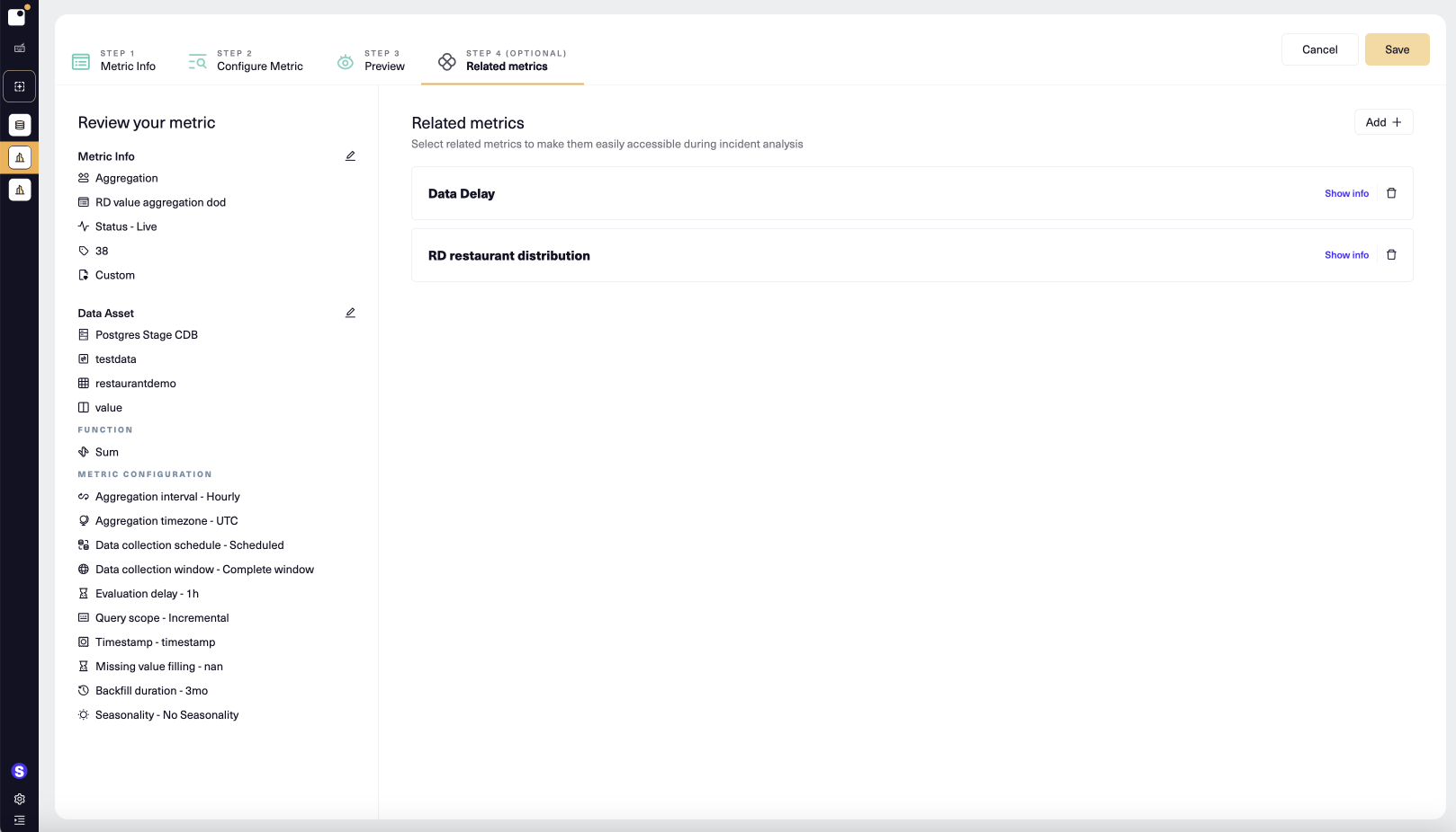
- To add a related metric, select Add + and then choose a metric in the listbox that appears.
- Select Show info inside a related metric to display the metric's ID and data asset(s).
- When you've added the related metrics you want, select Create (for a new metric) or Save.
- During incident analysis of the metric, any related metrics appear in the metrics listed on the left. You can then easily add them to the Metrics of interest, making the metric chart available within the incident.
Updated 10 months ago